In this post, we will generate populations of programs consisting of only eight instructions and optimize their fitness to reproduce a target behaviour (for example reversing a sequence) with genetic programming.

Genetic programming (GP) is a paradigm inspired by nature’s evolution process. It models a natural selection process of possible candidates. A research favorite in the last decade, because of its ability to derive macro-level behavior from plain description of micro-level interactions, it makes minimal assumption on the model structure and hence is applicable to a wide range of problems ¹.

I recently got two weeks of tinkering time and looked at interactions between an esoteric language and GP.

Zeroth order optimization with Crossovers and Mutations

First, we introduce some concepts for genetic programming, and model a problem interface with Rust’s trait syntax. The trait bundles all capabilities we expect from problems applicable to GP.

The GP implementation is generic over different problems and we provide necessary methods with trait bound P: Chromosome for the generic problem parameter P and trait Chromosome.

We will call possible solutions chromosomes , set of chromosomes our population, and the performance of a single chromose the fitness.

The key element of a genetic program is the ability to generate two (or more) offsprings from given parents. The method signature reads Chromosome::crossover(a: &Self, b: &Self) -> Vec<Self>; and generate combinations of features from both parents ².

Without mutation no new behavior could be introduced to our population. The Chromosome::mutate(self, p: f32) -> Self takes ownership of a chromosome and mutates its feature with a small probability p.

To keep well-working variations stable between iterations, we divide the population into two groups. The first is kept between iteration, the second is replaced and resampled based on fitness of the whole population.

Our algorithm is then pretty simple to lay out. We first assess our population based on the current fitness

let mut chromo_by_fitness = self.pops.drain(..).map(|c| (c, c.fitness()))
    .collect::<Vec<_>>();

chromo_by_fitness.sort_by(|a,b| a.1.total_cmp(&b.1));

we then keep the Nth best chromosomes in our population

let chroms = chromo_by_fitness.into_iter().map(|(c, _)| c).collect::<Vec<_>>();
self.pops.extend(chroms.into_iter().take(self.n_keep));

and replace the remaining population with offsprings from randomly sampled parents

let (parents_a, parents_b) = self.parents(&chromo_by_fitness, rng);

// perform crossovers
let childs = parents_a.into_iter().zip(parents_b.into_iter())
    .flat_map(|(a,b)| T::crossover(&chroms[a], &chroms[b], &mut rng))
    .collect::<Vec<_>>();

self.pops.extend(childs);

Finally, we introduce small random variations to our population set

self.pops = self.pops.into_iter().map(|x| T::mutate(x, &mut rng, self.mutation_p)).collect();

That provides us with a low number of hyper-parameters for the optimization process. We have the number of iterations, the total population size, the best population size and the mutation probability. We can add a small builder pattern to make configuration more simple, and have such a call procedure:

let pop: Population<Problem> = PopulationBuilder::default()
    .num_iter(500usize)
    .n_pop(16usize)
    .n_keep(8usize)
    .mutation_p(0.01)
    .build().unwrap()
    .execute(&mut rand::rng());

dbg!(&pop.get_best());

Function optimization

To make our algorithm more concrete, let’s implement a simple problem. We choose to optimize the Himmelblau’s function, a non-convex function with four minima and analytical solutions.

The performance of a chromosome is, in this example, simply the value of the function landscape at a point:

fn fitness(&self) -> f32 {
    (self.0.powf(2.0) + self.1 - 11.0).powf(2.0) + (self.0 + self.1.powf(2.0) - 7.).powf(2.0)
}

Performing a cross-over does a convex combinations of both 2D coordinates

fn crossover(x: &Self, y: &Self, rng: &mut Self::R) -> Vec<Self> {
    let uni = Uniform::new(0.0, 1.0).unwrap();
    let (a1, a2) = (uni.sample(rng), uni.sample(rng));
    let (b1, b2) = (uni.sample(rng), uni.sample(rng));

    vec![
        Self(x.0 * a1 + y.0 * (1. - a1), x.1 * a2 + y.1 * (1. - a2)), 
        Self(x.0 * b1 + y.0 * (1. - b1), x.1 * b2 + y.1 * (1. - b2))]
}

Random mutation adds noise to current solution to move outside of the solution space

fn mutate(mut self, rng: &mut Self::R, p: f32) -> Self {
    let uni = Uniform::new(-p, p).unwrap();
    self.0 += rng.sample(uni);
    self.1 += rng.sample(uni);

    self
}

Running this sample problem, yields the following sample progressions:

Esoteric language

For mathematical function optimization, genetic programming is ill equipped. If we increase the number of dimensions, our number of samples has to grow exponentially ³. But what we gain is flexibility in our problem definition. We will now see how to optimize a software function represented in the brainfuck (BF) language.

BF is a simplistic language which consists of only eigth instructions. It operates on a tape, and uses as simple input and output queue. The program and instruction definition of the AST reads as

type Program = Vec<Instruction>;

pub enum Instruction {
    Right,         // move pointer to the right for tape
    Left,          // move pointer to the left for tape
    Increment,     // increment value at current pointer
    Decrement,     // decrement value at current pointer
    Write,         // put current element to output
    Read,          // pop element to current pointer position
    Loop(Program), // loop until element is zero
}

Hence, due too its simple structure, implementing an interpreter is straightforward. ⁴

So how should a crossover or mutation function look like for a BF program? We should most certainly not apply them to the character-level representation, as they may be invalid due to mismatches between loop start [ and end ].

Instead, we traverse the instruction tree and mutate elements based on probability distributions. For mutation we randomly delete, replace a node at any position. Additionally, we also add a second node with a small probability to each position, so that the instruction tree can also grow. (and is actually balanced with chance of deletion).

let d = Bernoulli::new(p as f64).unwrap();
let instr = self.instr.into_iter()
    .filter_map(|mut ins| {
        // recurse into in case of a loop instruction
        if let Instruction::Loop(prg) = ins {
            ins = Instruction::Loop(prg.mutate(rng, p));
        }

        match (d.sample(rng), d.sample(rng), d.sample(rng)) {
            // drop at random
            (true, _, _) => None,
            // either generate insert second, or replace the current
            (false, true, _) | (false, false, true) => Some(Self::generate(1, rng).instr),
            // otherwise, just reuse the existing instruction
            (false, false, false) => Some(vec![ins]),
        }
    })
    .flatten()
    .collect();

The implementation of tree crossover is a bit more involved, but basically involves zipping both tree traversals and choosing either the node from tree A, or the tree of B at chance. It also handles edge-cases, when one tree is larger than another one.

let d = Bernoulli::new(0.95).unwrap();
let (mut var_a, mut var_b) = (Vec::new(), Vec::new());
for i in a.instr.iter().zip_longest(b.instr.iter()) {
    match i {
        Both(a,b) => {
            let (a,b) = match (a,b) {
                (Instruction::Loop(x), Instruction::Loop(y)) => {
                    let obj = Self::crossover(&x, &y, rng);

                    (Instruction::Loop(obj[0].clone()), Instruction::Loop(obj[1].clone()))
                },
                _ => (a.clone(),b.clone())
            };

            // whether we choose A or B for new A
            match d.sample(rng) {
                true => var_a.push(a.clone()),
                false => var_a.push(b.clone())
            }

            // whether we choose A or B for new B
            match d.sample(rng) {
                true => var_b.push(b.clone()),
                false => var_b.push(a.clone())
            }
        },
        Left(a) => // ...
        Right(b) => // ...
    }
}

Measuring program correctness

We generate pairs of random input and outputs. How do we measure the performance of our program for the give pairs? I choose the Levensthein distance for that.

The fitness function generates N samples with increasing length, generates the expected output, runs the program and compares the edit distance to the target.

fn fitness(&self) -> f32 {
    // init tape to max length of 512 bytes
    let mut tape = vec![0; 512];
    let mut idx = 256;

    // uniform distribution for input sampling
    let distr = Uniform::new(0, 255).unwrap();
    let rng = rand::rng();

    let mut samples = Vec::new();
    for i in 1..6 {
        // generate random input
        let inp = rng.clone().sample_iter(distr).take(i).map(|x| x as u8)
            .collect::<Vec<_>>();

        // run program 
        let res = self.run(&inp, &mut tape, &mut idx);

        // target is sequence reversal
        let target = inp.into_iter().rev()
            .collect::<Vec<_>>();

        // calculate edit distance
        samples.push(edit_distance(&res, &target) as f32);

        // reset tape
        tape = vec![0; 512];
        idx = 256;
    }

    // calculate sum of distance samples
    samples.into_iter().sum::<f32>()
}

Results of random permutations of programs

So, what is the chance that we are generating a working string reversal program after some iteration on our population:

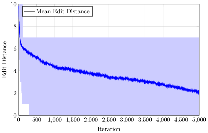
The figure highlights that we can find a working program after just 300 iterations, or we may be stuck without any progress for at least 5000 iterations. But on average our optimization process works and we can minimize the edit distance for 100 samples to around 2.

Conclusion

Mixing programs with some randomness and sorting results measured by some useful fitness, results in a working optimization process. Pretty neat. The process has of course some hyperparameters attached we have cross-validate, such as the population size, the mutation probability, but only a few. And for our simple problem of sequence reversal the average edit distance seems to be indeed monotonic decreasing.